Использование Статсмоделей для построения квантильной регрессии для полинома 2-го порядка
Я следую примеру StatsModels здесь, чтобы построить линии квантильной регрессии. С небольшими изменениями для моих данных пример отлично работает, производя этот график (обратите внимание, что я изменил код, чтобы построить только 0,05, 0,25, 0,5, 0,75 и 0,95 квантилей) :
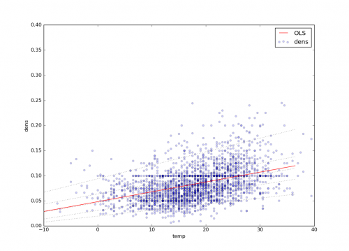
Однако я хотел бы построить OLS fit и соответствующие квантили для полиномиального fit 2-го порядка (вместо линейного). Например, вот строка OLS 2-го порядка для того же самого данные:
Как я могу изменить код в связанном примере для получения нелинейных квантилей?
Вот мой соответствующий код, модифицированный из связанного примера для получения 1-го участка:
d = {'temp': x, 'dens': y}
df = pd.DataFrame(data=d)

# Least Absolute Deviation
#
# The LAD model is a special case of quantile regression where q=0.5

mod = smf.quantreg('dens ~ temp', df)
res = mod.fit(q=.5)
print(res.summary())

# Prepare data for plotting
#
# For convenience, we place the quantile regression results in a Pandas DataFrame, and the OLS results in a dictionary.

quantiles = [.05, .25, .50, .75, .95]
def fit_model(q):
    res = mod.fit(q=q)
    return [q, res.params['Intercept'], res.params['temp']] + res.conf_int().ix['temp'].tolist()

models = [fit_model(x) for x in quantiles]
models = pd.DataFrame(models, columns=['q', 'a', 'b','lb','ub'])

ols = smf.ols('dens ~ temp', df).fit()
ols_ci = ols.conf_int().ix['temp'].tolist()
ols = dict(a = ols.params['Intercept'],
           b = ols.params['temp'],
           lb = ols_ci[0],
           ub = ols_ci[1])

print(models)
print(ols)

x = np.arange(df.temp.min(), df.temp.max(), 50)
get_y = lambda a, b: a + b * x

for i in range(models.shape[0]):
    y = get_y(models.a[i], models.b[i])
    plt.plot(x, y, linestyle='dotted', color='grey')

y = get_y(ols['a'], ols['b'])
plt.plot(x, y, color='red', label='OLS')

plt.scatter(df.temp, df.dens, alpha=.2)
plt.xlim((-10, 40))
plt.ylim((0, 0.4))
plt.legend()
plt.xlabel('temp')
plt.ylabel('dens')
plt.show()
1 ответ:
После целого дня изучения этого, пришел к решению, поэтому публикую свой собственный ответ. Большой кредит Йозеф Perktold в StatsModels для помощи.
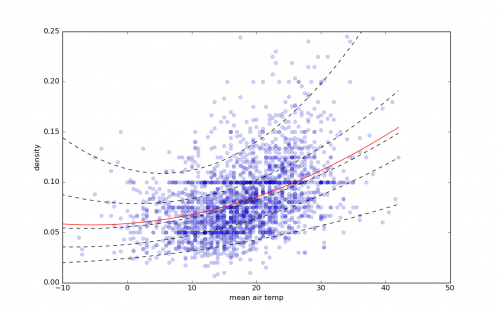
Вот соответствующий код и сюжет:
d = {'temp': x, 'dens': y}
df = pd.DataFrame(data=d)

x1 = pd.DataFrame({'temp': np.linspace(df.temp.min(), df.temp.max(), 200)})

poly_2 = smf.ols(formula='dens ~ 1 + temp + I(temp ** 2.0)', data=df).fit()
plt.plot(x, y, 'o', alpha=0.2)
plt.plot(x1.temp, poly_2.predict(x1), 'r-',
         label='2nd order poly fit, $R^2$=%.2f' % poly_2.rsquared,
         alpha=0.9)
plt.xlim((-10, 50))
plt.ylim((0, 0.25))
plt.xlabel('mean air temp')
plt.ylabel('density')
plt.legend(loc="upper left")


# with quantile regression

# Least Absolute Deviation
# The LAD model is a special case of quantile regression where q=0.5

mod = smf.quantreg('dens ~ temp + I(temp ** 2.0)', df)
res = mod.fit(q=.5)
print(res.summary())

# Quantile regression for 5 quantiles

quantiles = [.05, .25, .50, .75, .95]

# get all result instances in a list
res_all = [mod.fit(q=q) for q in quantiles]

res_ols = smf.ols('dens ~ temp + I(temp ** 2.0)', df).fit()


plt.figure()

# create x for prediction
x_p = np.linspace(df.temp.min(), df.temp.max(), 50)
df_p = pd.DataFrame({'temp': x_p})

for qm, res in zip(quantiles, res_all):
    # get prediction for the model and plot
    # here we use a dict which works the same way as the df in ols
    plt.plot(x_p, res.predict({'temp': x_p}), linestyle='--', lw=1,
             color='k', label='q=%.2F' % qm, zorder=2)

y_ols_predicted = res_ols.predict(df_p)
plt.plot(x_p, y_ols_predicted, color='red', zorder=1)
#plt.scatter(df.temp, df.dens, alpha=.2)
plt.plot(df.temp, df.dens, 'o', alpha=.2, zorder=0)
plt.xlim((-10, 50))
plt.ylim((0, 0.25))
#plt.legend(loc="upper center")
plt.xlabel('mean air temp')
plt.ylabel('density')
plt.title('')
plt.show()
Красная линия: полином 2-го порядка fit
Черные пунктирные линии: 5-й, 25-й, 50-й, 75-й, 95-й процентили